后训练量化（
PTQ
）在视觉
Transformer
（
ViTs
）领域引起了广泛关注，因为它在模型压缩方面表现出了高效率。然而，现有的方法通常忽视了量化权重和激活之间复杂的相互依赖关系，导致了相当大的量化误差。论文提出了一种名为
ERQ
的两步
PTQ
方法，精心设计用于顺序降低激活和权重量化带来的量化误差。
ERQ
首先引入了激活量化误差减小（
Aqer
），将激活量化误差的最小化策略性地表述为一个岭回归问题，并通过使用全精度更新权重来解决。随后，
ERQ
引入了权重量化误差减小（
Wqer
），采用迭代的方法来减轻由权重量化引起的量化误差。在每次迭代中，采用经验推导出的有效代理来细化量化权重的舍入方向，并结合岭回归求解器以减少权重量化误差。实验结果证明了该方法的有效性。值得注意的是，
ERQ
在
W3A4 ViT-S
的准确性上超越了最先进的
GPTQ
，提升幅度达
22.36%
。

来源：晓飞的算法工程笔记 公众号，转载请注明出处

论文: ERQ: Error Reduction for Post-Training Quantization of Vision Transformers

• 论文地址：
  https://arxiv.org/abs/2407.06794

Introduction

视觉
Transformer
（
ViTs
）显著挑战了卷积神经网络（
CNNs
），成为计算机视觉领域的新范式。
ViTs
利用多头自注意力（
MHSA
）机制来捕捉图像块之间的长距离关系，在各种视觉任务中展现出令人印象深刻的进展。

然而，强大的能力伴随着相当的复杂性。
ViTs
固有的架构复杂性导致了高计算需求和可观的内存要求，这在资源受限的环境中部署时带来了挑战。为了缓解这一困境，模型量化吸引了业界和学术界的持续关注。量化通过实现权重和激活的低位表示来减少模型复杂性，为高效部署提供了一条有前景的途径。最近，研究人员逐渐关注于视觉
Transformer
的后训练量化（
PTQ
），该方法旨在利用一个小型校准数据集和较低的成本对模型进行量化。

为了适应
ViTs
独特的结构，已经许多研究探索了各种后训练量化（
PTQ
）方法。例如，为了处理长尾
post-Softmax
激活，有研究提出了
\(log2/log \sqrt{2}\)
量化器和
twin uniform
量化器。为了管理高度变化的激活，有研究采用了重参数化技术和
power-of-two
因子。此外，有研究采用进化搜索方法来确定不稳定的缩放因子。然而，现有的方法通常忽视了权重和激活量化之间复杂的相互依赖关系，这在权重-激活量化时导致了相当大的量化误差。

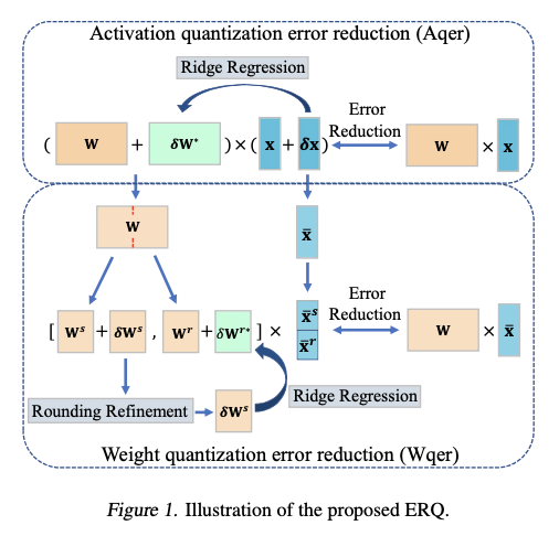
论文提出一种为
ViTs
量身定制的两步后训练量化方法
ERQ
，旨在顺序减小由量化激活和权重引起的量化误差。如图
1
所示，
ERQ
由两个步骤组成，即激活量化误差减少（
Aqer
）和权重量化误差减少（
Wqer
）。
Aqer
将激活量化引起的量化误差公式化为一个岭回归问题，该问题可以通过权重更新以闭式解的方式解决。随后，引入
Wqer
以迭代的量化和修正方式减小由权重量化引起的量化误差。特别地，在每次迭代中，量化全精度权重的前半部分，并通过先执行四舍五入细化，后再次解决岭回归问题来减小产生的量化误差。前者推导出输出误差的有效代理，用于细化量化权重的四舍五入方向，以降低量化误差。后者则通过更新剩余的全精度权重进一步减小量化误差。这样的过程持续进行，直到所有权重被准确量化。

ERQ
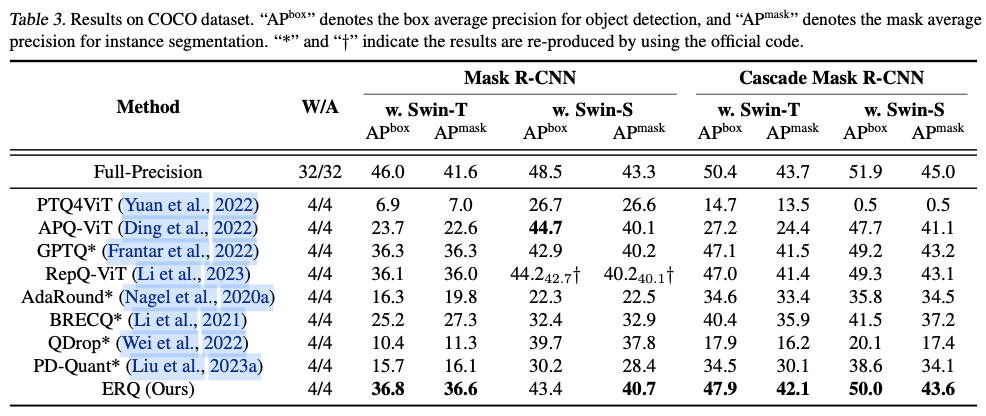
在对各种
ViTs
变体（
ViT
、
DeiT
和
Swin
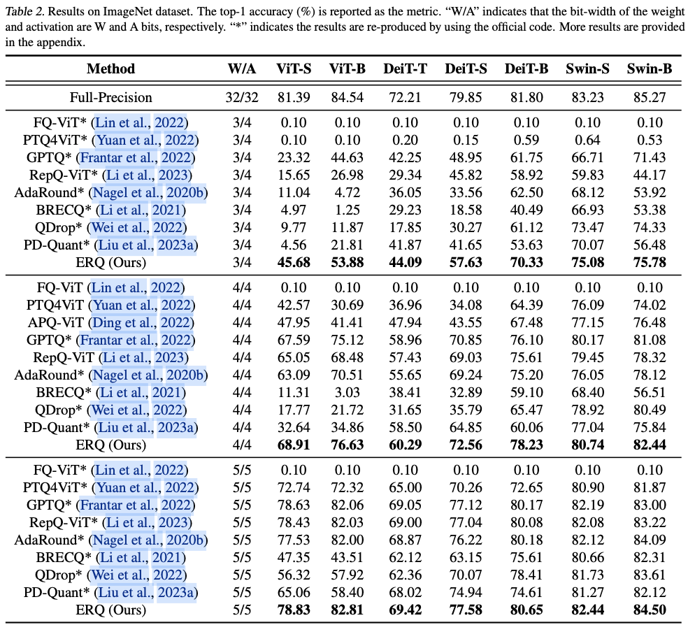
）及任务（图像分类、目标检测和实例分割）进行的广泛实验中证明了其有效性。值得注意的是，在图像分类任务中，
ERQ
在
W3A4 ViT-S
上比
GPTQ
的性能提高了
22.36%
。

Method

相互纠缠的
\(\delta{\mathbf{x}}\)
和
\(\delta\mathbf{W}\)
使得找到公式
4
的最优解变得具有挑战性。为使问题变得可处理，将公式
4
放宽为两个顺序的子问题，通过分别最小化来自量化激活和权重的误差。如图
1
所示，首先进行激活量化误差减少 (
Aqer
)，然后进行权重量化误差减少 (
Wqer
)。

Activation Quantization Error Reduction

为减轻由激活量化引起的误差，引入激活量化误差减少 (
Aqer
)，将误差减轻问题形式化为岭回归问题。具体来说，将权重保留为全精度，仅考虑由激活量化误差
\(\delta{\mathbf{x}}\)
引起的均方误差 (
MSE
)：

为了最小化公式
5
，将其形式化为岭回归问题，其中通过将权重
\(\mathbf{W}\)
与调整项
\(\delta\mathbf{W}^*\)
相加来完成最小化：

这里，
\(\delta\mathbf{W}^*\)
表示通过岭回归计算出的调整项，
\(\bar{\mathbf{x}}=\mathbf{x}+\delta\mathbf{x}\)
是量化输入，
\(\lambda_1\| \delta\mathbf{W}^* \|_2^2\)
作为正则化项，
\(\lambda_1\)
是控制正则化强度的超参数。公式
6
构成了岭回归问题。为了最小化它，首先计算其相对于
\(\delta\mathbf{W}^*\)
的梯度：

然后，通过将公式
7
设置为零来求解
\(\delta\mathbf{W}^*\)
：

正则化项
\(\lambda_1 \mathbf{I}\)
确保
\(\mathbb{E} \left[\bar{\mathbf{x}}\bar{\mathbf{x}}^T \right] + \lambda_1 \mathbf{I}\)
的逆始终存在，这对计算稳定性至关重要。此外，它抑制了异常值，从而减轻了过拟合，提高了模型的泛化能力。抑制异常值对于随后的权重量化也至关重要，因为它限制了权重的范围。这种限制防止量化点分布在未覆盖的区域，从而增强了量化的表达能力。

在实践中，给定校准数据集，使用
\(\frac{1}{N}\sum_n^N \delta{\mathbf{x}}_n\bar{\mathbf{x}}_n^T\)
和
\(\frac{1}{N}\sum_n^N \bar{\mathbf{x}}_n\bar{\mathbf{x}}_n^T\)
分别估计
\(\mathbb{E}\left[\delta{\mathbf{x}}\bar{\mathbf{x}}^T\right]\)
和
\(\mathbb{E}\left[\bar{\mathbf{x}}\bar{\mathbf{x}}^T \right]\)
。这里，
\(N = B\times T >> D_{in}^s\)
，其中
\(B\)
是校准数据集的大小，
\(T\)
是一张图像的标记数量。请注意，
\(\delta{\mathbf{x}}\)
和
\(\bar{\mathbf{x}}\)
是在给定输入和量化参数的情况下确定的。在得到
\(\delta\mathbf{W}^*\)
后，通过
\(\mathbf{W} = \mathbf{W} + \delta\mathbf{W}^*\)
将其合并到网络的权重中。通过这样做，所提出的
Aqer
明确减轻了从量化激活到权重的量化误差。

Weight Quantization Error Reduction

在进行
Aqer
后需执行权重量化，提出权重量化误差减少（
Wqer
）来减轻由此产生的量化误差。在这里，目标被定义为：

注意，在进行
Aqer
后，激活值被量化。公式
9
表明输出通道之间的最小化是独立进行的。因此，分别分析每个
\(\mathcal{L}^{\text{MSE}}_i\)
的最小化。同时对整个全精度权重进行量化会导致无法恢复的量化误差。因此，采用迭代的量化和修正方法，逐步减少由权重量化引起的量化误差。

在每次迭代中，首先对未量化权重的前半部分进行量化，然后减轻由此产生的量化误差。具体来说，从当前的全精度权重
\(\mathbf{W}_{i,:}\)
和相应的
\(\bar{\mathbf{x}}\)
开始。然后，将
\(\mathbf{W}\)
划分为两个部分：前半部分
\(\mathbf{W}^s_{i,:} \in \mathbb{R}^{ 1\times D_{in}^s}\)
用于量化，而剩余部分
\(\mathbf{W}^r_{i,:} \in \mathbb{R}^{1 \times D_{in}^r}\)
保持全精度。对应地，从
\(\bar{\mathbf{x}}\)
中派生出
\(\bar{\mathbf{x}}^s \in \mathbb{R}^{D_{in}^s}\)
和
\(\bar{\mathbf{x}}^r \in \mathbb{R}^{D_{in}^r}\)
，其中
\(\bar{\mathbf{x}}^s\)
和
\(\bar{\mathbf{x}}^r\)
分别包含与
\(\mathbf{W}^s_{i,:}\)
和
\(\mathbf{W}^r_{i,:}\)
对应的
\(\bar{\mathbf{x}}\)
的行。量化后的
\(\mathbf{W}^s_{i,:}\)
的量化误差记为
\(\delta\mathbf{W}^s_{i,:} = \bar{\mathbf{W}}^s_{i,:} - \mathbf{W}^s_{i,:}\)
，由此产生的均方误差（
MSE
）为：

在这里，
\(\mathbf{W}_{i,:} = [ \mathbf{W}^s_{i,:},\mathbf{W}^r_{i,:} ]\)
，
\(\bar{\mathbf{x}} = [ \bar{\mathbf{x}}^s, \bar{\mathbf{x}}^r ]\)
。为了减轻公式
10
，首先引入四舍五入优化（
Rounding Refinement
），在该过程中会细化量化权重的四舍五入方向。比如调整
\(\delta\mathbf{W}^s_{i,:}\)
，以减少
\(\mathbb{E} \left[ \| \delta\mathbf{W}^s_{i,:}\bar{\mathbf{x}}^s \|_2^2 \right]\)
本身。然后，在四舍五入优化之后，给定
\(\mathbb{E} \left[ \| \delta\mathbf{W}^s_{i,:}\bar{\mathbf{x}}^s \|_2^2 \right]\)
，构建一个岭回归（
Ridge Regression
）问题，通过调整
\(\mathbf{W}^r_{i, :}\)
来进一步减轻该误差。

Rounding Refinement

最初，目标是调整量化权重的四舍五入方向，以最小化
\(\mathbb{E} \left[ \| \delta\mathbf{W}^s_{i,:}\bar{\mathbf{x}}^s \|_2^2 \right]\)
。具体来说，对于
\(\mathbf{W}^s_{i,:}\)
中的第
\(j\)
个值，记作
\(\mathbf{W}^s_{i,j}\)
，量化过程涉及向下取整或向上取整。因此，
\(\mathbf{W}^s_{i,:}\)
的量化误差，记作
\(\delta\mathbf{W}^s_{i,j}\)
，可以表示为
\(\delta\mathbf{W}^{s\downarrow}{i, j}\)
或
\(\delta\mathbf{W}^{s\uparrow}{i, j}\)
。这里，
\(\delta\mathbf{W}^{s\downarrow}_{i, j} = \mathbf{W}^s_{i,j} - \text{Q}_{un\downarrow}(\mathbf{W}^s_{i,j}, b) > 0\)
表示采用向下取整策略所产生的误差，
\(\delta\mathbf{W}^{s\uparrow}_{i, j} = \mathbf{W}^s_{i,j} - \text{Q}_{un\uparrow}(\mathbf{W}^s_{i,j}, b) < 0\)
表示采用向上取整策略所产生的误差，其中
\(\downarrow/\uparrow\)
表示在公式
1
中将
\(\left\lfloor \cdot \right\rceil\)
替换为
\(\left\lfloor \cdot \right\rfloor\)
/
\(\left\lceil \cdot \right\rceil\)
。

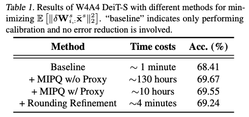
选择
\(\delta\mathbf{W}^s_{i,:}\)
是一个
NP
难题，其解可以通过混合整数二次规划（
MIPQ
）进行搜索。然而，
\(\mathbb{E} \left[ \| \delta\mathbf{W}^s_{i,:}\bar{\mathbf{x}}^s \|_2^2 \right]\)
的高计算复杂度使得在合理时间内找到解决方案成为一项挑战。如表
1
所示，使用
\(\mathbb{E} \left[ \| \delta\mathbf{W}^s_{i,:}\bar{\mathbf{x}}^s \|_2^2 \right]\)
作为
MIPQ
的目标消耗了约
130
小时的巨大时间成本。

• Efficient Proxy

因此，目标是找到
\(\mathbb{E} \left[ \| \delta\mathbf{W}^s_{i,:}\bar{\mathbf{x}}^s \|_2^2 \right]\)
的一个高效代理。首先，将
\(\mathbb{E} \left[ \| \delta\mathbf{W}^s_{i,:}\bar{\mathbf{x}}^s \|_2^2 \right]\)
重写为：

这里，
\(\Delta\)
表示利用
\(\mathbb{E}\left[ Z^2 \right] = (\mathbb{E}\left[ Z \right])^2 + \text{Var}\left[ Z \right]\)
。

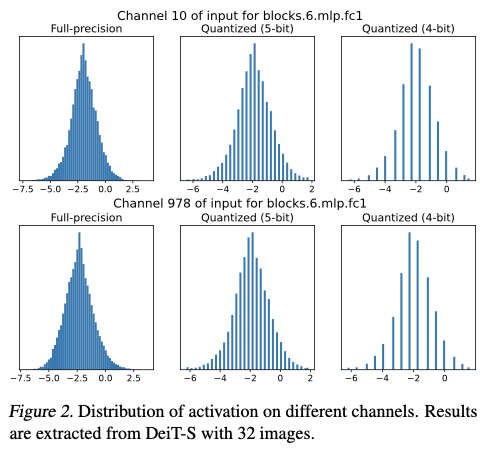
根据中心极限定理，神经网络中的大量乘法和加法运算使得激活值通常呈现出高斯分布，这也是许多以前量化领域研究的基本假设。同时，图
2
展示了全精度和量化激活的通道分布。可以看出，量化激活仍然表现出近似的高斯分布。

因此，论文认为
\(\bar{\mathbf{x}}^s\)
的通道分布仍然可以通过高斯分布进行捕捉，并用
\(D_{in}^s\)
维的高斯分布
\(\mathcal{N}(\boldsymbol{\mu}^s, \boldsymbol{\Sigma}^s)\)
对
\(\bar{\mathbf{x}}^s\)
进行建模，其中
\(D_{in}^s\)
是
\(\bar{\mathbf{x}}^s\)
的维度，
\(\boldsymbol{\mu}^s \in \mathbb{R}^{D_{in}^s}, \boldsymbol{\Sigma}^s \in \mathbb{R}^{D_{in}^s \times D_{in}^s}\)
。然后，公式
11
变为：

这里，公式
12
是得到的
\(\mathbb{E} \left[ \| \delta\mathbf{W}^s_{i,:}\bar{\mathbf{x}}^s \|_2^2 \right]\)
的代理。在实践中，使用给定的校准数据集来估计经验值
\(\hat{\boldsymbol{\mu}}^s\)
和
\(\hat{\boldsymbol{\Sigma}}^s\)
。请注意，对于所有输出通道，
\(\hat{\boldsymbol{\mu}}^s\)
和
\(\hat{\boldsymbol{\Sigma}}^s\)
是共享的，只需进行一次计算。

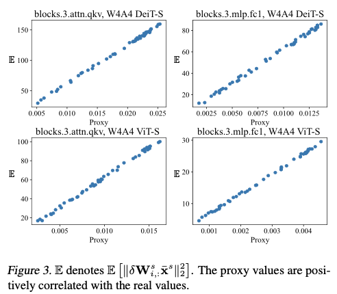
图
3
展示了代理与
\(\mathbb{E} \left[ \| \delta\mathbf{W}^s_{i,:}\bar{\mathbf{x}}^s \|_2^2 \right]\)
之间的关系。可以看出，所提出的代理与真实值成比例，证明了其可信度。

使用代理的计算复杂度为
\(O((D_{in}^s)^2)\)
，而
\(\mathbb{E} \left[ \| \delta\mathbf{W}^s_{i,:}\bar{\mathbf{x}}^s \|_2^2 \right]\)
的复杂度为
\(O(ND_{in}^s)\)
，其中
\(N >> D_{in}^s\)
。因此，该代理可以作为一个低成本的目标，用于求解
\(\delta\mathbf{W}^s_{i,:}\)
。如表
1
所示，将方程
12
作为
MIPQ
的目标将时间成本从约
130
小时降低到约
10
小时。然而，由于当前开源的
MIPQ
实现仅支持
CPU
，无法充分利用
GPU
的能力，这样的成本仍然是适度的。接下来将介绍
Rounding Refinement
，一种支持
GPU
的方法，利用代理的梯度更快地调整
\(\delta\mathbf{W}^s_{i,:}\)
。

• Rounding Refinement

首先，使用最接近取整策略初始化
\(\delta\mathbf{W}^s_{i,j}\)
。此时，
\(\delta\mathbf{W}^s_{i,j}\)
要么等于
\(\delta\mathbf{W}^{s\downarrow}_{i, j}\)
，要么等于
\(\delta\mathbf{W}^{s\uparrow}_{i, j}\)
。然后，目标是确定一个索引集合
\(\mathcal{S}\)
，该集合包含需要修改的元素的索引集合，其取整方向被颠倒：

为了确定
\(\mathcal{S}\)
，首先对代理（公式
12
）相对于
\(\delta\mathbf{W}^s_{i,:}\)
求导。

只选择梯度符号相同的元素，因为这才是允许颠倒的唯一方式。例如，当
\(\delta\mathbf{W}_{i, j}^s = \delta\mathbf{W}^{s\downarrow}_{i, j}\)
时，仅当
\(\boldsymbol{G}_{\delta\mathbf{W}_{i, j}^s}\)
与
\(\delta\mathbf{W}_{i, j}^s\)
具有相同的符号时，才能将其替换为
\(\delta\mathbf{W}^{s\uparrow}_{i, j}\)
。因此，索引集合
\(\mathcal{S}\)
定义为：

这里，
\(\mathrm{topk\_index}\)
返回前
\(\mathrm{k}\)
个元素的索引，
\(\mathbb{1}(\cdot)\)
对于非负输入返回
1
，对负输入返回
0
，
\(\lvert \cdot \rvert\)
返回输入的绝对值。

在获得
\(\mathcal{S}\)
后，通过公式
13
进行颠倒。上述过程会迭代，直到调整后的
\(\delta\mathbf{W}^s_{i, :}\)
引发更大的代理值或达到最大迭代次数。在获得
\(\delta\mathbf{W}^s_{i, :}\)
后，量化可以通过
\(\bar{\mathbf{W}}^s_{i, :} = \mathbf{W}^s_{i, :}+\delta\mathbf{W}^s_{i, :}\)
完成。然后，将
\(\bar{\mathbf{W}}^s_{i, :}\)
添加到量化权重集合中。
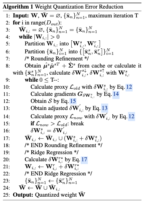
Rounding Refinement
的整体过程在算法
1
的第
7
行到第
18
行中给出。如表
1
所示，
Rounding Refinement
通过
\(150\times\)
的成本显著减少了时间开销，从
10
小时减少到
4
分钟，同时可接受的准确性损失。

• Ridge Regression

在
Rounding Refinement
之后，建议用
\(\delta\mathbf{W}^{r*}_{i, :}\)
调整
\(\mathbf{W}^r_{i, :}\)
，以进一步抵消
\(\mathbb{E} \left[ \| \delta\mathbf{W}^s_{i,:}\bar{\mathbf{x}}^s \|_2^2 \right]\)
，从而得到以下目标：

其中，
\(\lambda_2\)
是一个超参数，用于控制正则化项
\(\lambda_2\| \delta\mathbf{W}^{r*}_{i, :} \|_2^2\)
的强度。公式
16
的最小化形成了岭回归问题，解决方案定义为：

在实践中，通过使用
\(\frac{1}{N}\sum_n^N \bar{\mathbf{x}}_n^r\bar{\mathbf{x}}_n^{sT}\)
和
\(\frac{1}{N}\sum_n^N \bar{\mathbf{x}}_n^r\bar{\mathbf{x}}_n^{rT}\)
来估计
\(\mathbb{E}\left[\bar{\mathbf{x}}^r \bar{\mathbf{x}}^{sT}\right]\)
和
\(\mathbb{E}\left[\bar{\mathbf{x}}^r \bar{\mathbf{x}}^{rT} \right]\)
。随后，
\(\mathbf{W}^r_{i, :} = \mathbf{W}^r_{i, :}+\delta\mathbf{W}^{r*}_{i, :}\)
以减小误差。目前，
\(\mathbf{W}^r_{i, :}\)
仍然保持为全精度，并将在下一次迭代中处理。该过程持续进行，直到所有权重被准确量化。所提出的
Rounding Refinement
和
Ridge Regression
共同形成了
Wqer
，其整体过程在算法
1
中给出。在实践中，对多个输出通道并行执行
Wqer
。

Experiments

如果本文对你有帮助，麻烦点个赞或在看呗～
更多内容请关注 微信公众号【晓飞的算法工程笔记】